Reanalyzing the Schnall/Johnson “cleanliness” data sets: New insights from Bayesian and robust approaches

I want to present a re-analysis of the raw data from two studies that investigated whether physical cleanliness reduces the severity of moral judgments – from the original study (n = 40; Schnall, Benton, & Harvey, 2008), and from a direct replication (n = 208, Johnson, Cheung, & Donnellan, 2014). Both data sets are provided on the Open Science Framework. All of my analyses are based on the composite measure as dependent variable.

This re-analsis follows previous analyses by Tal Yarkoni, Yoel Inbar, and R. Chris Fraley, and is focused on one question: What can we learn from the data when we apply modern (i.e., Bayesian and robust) statistical approaches?
The complete and reproducible R code for these analyses is at the end of the post.

Disclaimer 1: This analysis assumes that the studies from which data came from were internally valid. Of course the garbage-in-garbage-out principle holds. But as the original author reviewed the experimental material of the replication study and gave her OK, I assume that the relication data is as valid as the original data.
Disclaimer 2: I am not going to talk about tone, civility, or bullying here. Although these are important issues, a lot has been already written about it, including apologies from one side of the debate (not from the other, yet), etc. For nice overviews over the debate, see for example a blog post by Vasudevan Mukunth, and the summary provided by Tal Yarkoni). I am completely unemotional about these data. False positives do exists, I am sure I had my share of them, and replication is a key element of science. I do not suspect anybody of anything – I just look at the data.
That being said, let’s get to business:

Bayes factor analysis

The BF is a continuous measure of evidence for H0 or for H1, and quantifies, “how much more likely is H1 compared to H0″. Typically, a BF of at least 3 is requested to speak of evidence (i.e., the H1 should be at least 3 times more likely than the H0 to speak of evidence for an effect). For an introduction to Bayes factors see here, here, or here.
Using the BayesFactor package, it is simple to compute a Bayes factor (BF) for the group comparison. In the original study, the Bayes factor against the H0, , is 1.08. That means, data are 1.08 times more likely under the H1 (“there is an effect”) than under the H0 (“There is no effect”). As the BF is virtually 1, data occurred equally likely under both hypotheses.

What researchers actually are interested in is not p(Data | Hypothesis), but rather p(Hypothesis | Data). Using Bayes’ theorem, the former can be transformed into the latter by assuming prior probabilities for the hypotheses. The BF then tells one how to update one’s prior probabilities after having seen the data. Given a BF very close to 1, one does not have to update his or her priors. If one holds, for example, equal priors (p(H1) = p(H0) = .5), these probabilities do not change after having seen the data of the original study. With these data, it is not possible to decide between H0 and H1, and being so close to 1, this BF is not even “anectdotal evidence” for H1 (although the original study was just skirting the boundary of significance, p = .06).

For the replication data, the situation looks different. The Bayes factor  here is 0.11. That means, H0 is (1 / 0.11) = 9 times more likely than H1. A  of 0.11 would be labelled “moderate to strong evidence” for H0. If you had equals priors before, you should update your belief for H1 to 10% and for H0 to 90% (Berger, 2006).
To summarize, neither the original nor the replication study show evidence for H1. In contrast, the replication study even shows quite strong evidence for H0.

A more detailed look at the data using robust statistics

Parametric tests, like the ANOVA employed in the original and the replication study, rest on assumptions. Unfortunately, these assumptions are very rarely met (Micceri, 1989), and ANOVA etc. are not as robust against these violations as many textbooks suggest (Erceg-Hurn & Mirosevic, 2008). Fortunately, over the last 30 years robust statistical methods have been developed that do not rest on such strict assumptions.

In the presence of violations and outliers, these robust methods have much lower Type I error rates and/or higher power than classical tests. Furthermore, a key advantage of these methods is that they are designed in a way that they are equally efficient compared to classical methods, even if the assumptions are not violated. In a nutshell, when using robust methods, there nothing to lose, but a lot to gain.
Rand Wilcox pioneered in developing many robust methods (see, for example, this blog post by him), and the methods are implemented in the WRS package for R (Wilcox & Schönbrodt, 2014).

Comparing the central tendency of two groups

A robust alternative to the independent group t test would be to compare the trimmed means via percentile bootstrap. This method is robust against outliers and does not rest on parametric assumptions. Here we find a p value of .106 for the original study and p = .94 for the replication study. Hence, the same picture: No evidence against the H0.

Comparing other-than-central tendencies between two groups, aka.: Comparing extreme quantiles between groups

When comparing data from two groups, approximately 99.6% of all psychological research compares the central tendency (that is a subjective estimate). In some cases, however, it would be sensible to compare other parts of the distributions.For example, an intervention could have effects only on slow reaction times (RT), but not on fast or medium RTs. Similarly, priming could have an effect only on very high responses, but not on low and average responses. Measures of central tendency might obscure or miss this pattern.

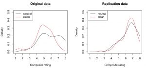
And indeed, descriptively there (only) seems to be a priming effect in the “extremely wrong pole” (large numbers on the x axis) of the original study (i.e., the black density line is higher than the red on at “7” and “8” ratings):

This visual difference can be tested. Here, I employed the [cci]qcomhd[/cci] function from the WRS package (Wilcox, Erceg-Hurn, Clark, & Carlson, 2013). This method looks whether two samples differ in several quantiles (not only the central tendency). For an introduction to this method, see this blog post.

Here’s the result when comparing the 10th, 30th, 50th, 70th, and 90th quantile:
[cc lang=”rsplus” escaped=”true”]
q n1 n2 est.1 est.2 est.1_minus_est.2 ci.low ci.up p_crit p.value signif
1 0.1 20 20 3.86 3.15 0.712 -1.077 2.41 0.0500 0.457 NO
2 0.3 20 20 4.92 4.51 0.410 -0.341 1.39 0.0250 0.265 NO
3 0.5 20 20 5.76 5.03 0.721 -0.285 1.87 0.0167 0.197 NO
4 0.7 20 20 6.86 5.70 1.167 0.023 2.05 0.0125 0.047 NO
5 0.9 20 20 7.65 6.49 1.163 0.368 1.80 0.0100 0.008 YES
[/cc]
(Please note: Estimating 5 quantiles from 20 data points is not quite the epitome of precision. So treat this analysis with caution.)

As multiple comparison are made, the Benjamini-Hochberg-correction for the p value is applied. This correction gives new critical p values (column [cci]p_crit[/cci]) to which the actual p values (column [cci]p.value[/cci]) have to be compared. One quantile survives the correction: the 90th quantile. That means that there are fewer extreme answers in the cleanliness priming group than in the control group. This finding, of course, is purely exploratory, and as any other exploratory finding it awaits cross-validation in a fresh data set. Luckily, we have the replication data set! Let’s see whether we can replicate this effect.

The answer is: no. Not even a tendency:

[cc lang=”rsplus” escaped=”true”]
q n1 n2 est.1 est.2 est.1_minus_est.2 ci.low ci.up p_crit p.value signif
1 0.1 102 106 4.75 4.88 -0.1309 -0.705 0.492 0.0125 0.676 NO
2 0.3 102 106 6.00 6.12 -0.1152 -0.571 0.386 0.0250 0.699 NO
3 0.5 102 106 6.67 6.61 0.0577 -0.267 0.349 0.0500 0.737 NO
4 0.7 102 106 7.11 7.05 0.0565 -0.213 0.411 0.0167 0.699 NO
5 0.9 102 106 7.84 7.73 0.1111 -0.246 0.431 0.0100 0.549 NO
[/cc]
Here’s a plot of the results:

Overall summary

From the Bayes factor analysis, both the original and the replication study do not show evidence for the H1. The replication study actually shows moderate to strong evidence for the H0.

If anything, the original study shows some exploratory evidence that only the high end of the answer distribution (around the 90th quantile) is reduced by the cleanliness priming – not the central tendency. If one wants to interpret this effect, it would translate to: “Cleanliness primes reduce extreme morality judgements (but not average or low judgements)”. This exploratory effect, however, could not be cross-validated in the better powered replication study.

Outlook

Recently, Silberzahn, Uhlmann, Martin, and Nosek proposed “crowdstorming a data set”, in cases where a complex data set calls for different analytical approaches. Now, a simple two group experimental design, usually analyzed with a t test, doesn’t seem to have too much complexity – still it is interesting how different analytical approaches highlight different aspects of the data set. And it is also interesting to see that the majority of diverse approaches comes to the same conclusion: From this data base, we can conclude that we cannot conclude that the H0 is wrong (This sentence, a hommage to Cohen, 1990, was for my Frequentist friends ;-)).

And, thanks to Bayesian approaches, we can say (and even understand): There is strong evidence that the H0 is true. Very likely, there is no priming effect in this paradigm.

PS: Celebrate open science. Without open data, all of this would not be possible.

[cc lang=”rsplus” escaped=”true” collapse=”true”]
## (c) 2014 Felix Schönbrodt
## https://www.nicebread.de
##
## This is a reanalysis of raw data from
## – Schnall, S., Benton, J., & Harvey, S. (2008). With a clean conscience cleanliness reduces the severity of moral judgments. Psychological Science, 19(12), 1219-1222.
## – Johnson, D. J., Cheung, F., & Donnellan, M. B. (2014). Does Cleanliness Influence Moral Judgments? A Direct Replication of Schnall, Benton, and Harvey (2008). Social Psychology, 45, 209-215.
## ======================================================================
## Read raw data, provided on Open Science Framework
# – https://osf.io/4cs3k/
# – https://osf.io/yubaf/
## ======================================================================
library(foreign)
dat1 <- read.spss(“raw/Schnall_Benton__Harvey_2008_Study_1_Priming.sav”, to.data.frame=TRUE) dat2 <- read.spss(“raw/Exp1_Data.sav”, to.data.frame=TRUE) dat2 <- dat2[dat2[, “filter_.”] == “Selected”, ] dat2$condition <- factor(dat2$Condition, labels=c(“neutral priming”, “clean priming”)) table(dat2$condition) # build composite scores from the 6 vignettes: dat1$DV <- rowMeans(dat1[, c(“dog”, “trolley”, “wallet”, “plane”, “resume”, “kitten”)]) dat2$DV <- rowMeans(dat2[, c(“Dog”, “Trolley”, “Wallet”, “Plane”, “Resume”, “Kitten”)]) # define shortcuts for DV in each condition neutral <- dat1$DV[dat1$condition == “neutral priming”] clean <- dat1$DV[dat1$condition == “clean priming”] neutral2 <- dat2$DV[dat2$condition == “neutral priming”] clean2 <- dat2$DV[dat2$condition == “clean priming”] ## ====================================================================== ## Original analyses with t-tests/ ANOVA ## ====================================================================== # ——————————————————————— # Original study: # Some descriptives … mean(neutral) sd(neutral) mean(clean) sd(clean) # Run the ANOVA from Schnall et al. (2008) a1 <- aov(DV ~ condition, dat1) summary(a1) # p = .0644 # –> everything as in original publication
# ———————————————————————
# Replication study
mean(neutral2)
sd(neutral2)
mean(clean2)
sd(clean2)
a2 <- aov(DV ~ condition, dat2) summary(a2) # p = .947 # –> everything as in replication report
## ======================================================================
## Bayes factor analyses
## ======================================================================
library(BayesFactor)
ttestBF(neutral, clean, rscale=1) # BF_10 = 1.08
ttestBF(neutral2, clean2, rscale=1) # BF_10 = 0.11
## ======================================================================
## Robust statistics
## ======================================================================
library(WRS)
# ———————————————————————
# robust tests: group difference of central tendency
# percentile bootstrap for comparing measures of location:
# 20% trimmed mean
trimpb2(neutral, clean) # p = 0.106 ; CI: [-0.17; +1.67]
trimpb2(neutral2, clean2) # p = 0.9375; CI: [-0.30; +0.33]
# median
medpb2(neutral, clean) # p = 0.3265; CI: [-0.50; +2.08]
medpb2(neutral2, clean2) # p = 0.7355; CI: [-0.33; +0.33]
# ———————————————————————
# Comparing other quantiles (not only the central tendency)
# plot of densities
par(mfcol=c(1, 2))
plot(density(clean, from=1, to=8), ylim=c(0, 0.5), col=”red”, main=”Original data”, xlab=”Composite rating”)
lines(density(neutral, from=1, to=8), col=”black”)
legend(“topleft”, col=c(“black”, “red”), lty=”solid”, legend=c(“neutral”, “clean”))
plot(density(clean2, from=1, to=8), ylim=c(0, 0.5), col=”red”, main=”Replication data”, xlab=”Composite rating”)
lines(density(neutral2, from=1, to=8), col=”black”)
legend(“topleft”, col=c(“black”, “red”), lty=”solid”, legend=c(“neutral”, “clean”))
# Compare quantiles of original study …
par(mfcol=c(1, 2))
qcomhd(neutral, clean, q=seq(.1, .9, by=.2), xlab=”Original: Neutral Priming”, ylab=”Neutral – Clean”)
abline(h=0, lty=”dotted”)
# Compare quantiles of replication study
qcomhd(neutral2, clean2, q=seq(.1, .9, by=.2), xlab=”Replication: Neutral Priming”, ylab=”Neutral – Clean”)
abline(h=0, lty=”dotted”)
[/cc]
References
Berger, J. O. (2006). Bayes factors. In S. Kotz, N. Balakrishnan, C. Read, B. Vidakovic, & N. L. Johnson (Eds.), Encyclopedia of Statistical Sciences, vol. 1 (2nd ed.) (pp. 378–386). Hoboken, NJ: Wiley.
Erceg-Hurn, D. M., & Mirosevich, V. M. (2008). Modern robust statistical methods: An easy way to maximize the accuracy and power of your research. American Psychologist, 63, 591–601.
Micceri, T. (1989). The unicorn, the normal curve, and other improbable creatures. Psychological Bulletin, 105, 156–166. doi:10.1037/0033-2909.105.1.156
Schnall, S., Benton, J., & Harvey, S. (2008). With a clean conscience cleanliness reduces the severity of moral judgments. Psychological Science, 19(12), 1219–1222.
Wilcox, R. R., Erceg-Hurn, D. M., Clark, F., & Carlson, M. (2013). Comparing two independent groups via the lower and upper quantiles. Journal of Statistical Computation and Simulation, 1–9. doi:10.1080/00949655.2012.754026
Wilcox, R.R., & Schönbrodt, F.D. (2014). The WRS package for robust statistics in R (version 0.25.2). Retrieved from https://github.com/nicebread/WRS