
Summary: A new function in the WRS package compares many quantiles of two distributions simultaneously while controlling the overall alpha error.
When comparing data from two groups, approximately 99.6% of all psychological research compares the central tendency (that is a subjective estimate).
In some cases, however, it would be sensible to compare different parts of the distributions. For example, in reaction time (RT) experiments two groups may only differ in the fast RTs, but not in the long. Measures of central tendency might obscure or miss this pattern, as following example demonstrates.
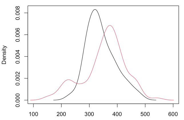
Imagine RT distributions for two experimental conditions (“black” and “red”). Participants in the red condition have some very fast RTs:
[cc lang=”rsplus” escaped=”true”]set.seed(1234)
RT1 <- rnorm(100, 350, 52)
RT2 <- c(rnorm(85, 375, 55), rnorm(15, 220, 25))
plot(density(RT1), xlim=c(100, 600))
lines(density(RT2), col=2)[/cc]
A naïve (but common) approach would be to compare both distributions with a t test:
data: RT1 and RT2
t = -1.3219, df = 175.21, p-value = 0.1879
alternative hypothesis: true difference in means is not equal to 0
95 percent confidence interval:
-30.442749 6.019772
sample estimates:
mean of x mean of y
341.8484 354.0599
Results show that both groups do not differ in their central tendency.
Now let’s do the same with a new method!
The function qcomhd from the WRS package compares user-defined quantiles of both distributions using a Harrell–Davis estimator in conjunction with a percentile bootstrap. The method seems to improve over other methods: “Currently, when there are tied values, no other method has been found that performs reasonably well. Even with no tied values, method HD can provide a substantial gain in power when q ≤ .25 or q ≥ .75 compared to other techniques that have been proposed”. The method is described in the paper “Comparing two independent groups via the upper and lower quantiles” by Wilcox, Erceg-Hurn, Clark and Carlson (2013).
You can use the function as soon as you install the latest version of the WRS package following this installation instruction.
Let’s compare all percentiles from the 10th to the 90th:qcomhd(RT1, RT2, q = seq(.1, .9, by=.1))
The graphical output shows how groups differ in the requested quantiles, and the confidence intervals for each quantile:
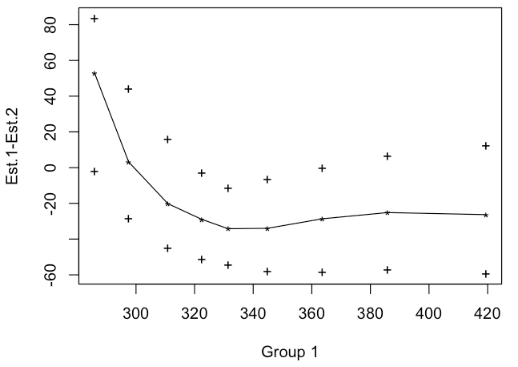
The text output (see below) also shows that groups differ significantly in the 40th, the 50th, 60th and the 70th percentile. The column labeled ‘’p.value’’ shows the p value for a single quantile bootstrapping test. As we do multiple tests (one for each quantile), the overall Type 1 error (defaulting to .05) is controlled by the Hochberg method. Therefore, for each p value a critical p value is calculated that must be undercut (see column ‘_crit’. The column ‘signif’ marks all tests which fulfill this condition:
    q  n1  n2    est.1    est.2 est.1_minus_est.2     ci.low       ci.up      p_crit p.value signif
1 0.1 100 100 285.8276 232.7603         53.067277  -1.935628  83.7476155 0.010000000   0.015     NO
2 0.2 100 100 297.5061 294.3337          3.172353 -28.192629  44.0262212 0.050000000   0.842     NO
3 0.3 100 100 310.8760 331.0405        -20.164536 -44.904146  15.8367276 0.016666667   0.131     NO
4 0.4 100 100 322.5014 351.4840        -28.982614 -51.051513  -2.7466374 0.007142857   0.003    YES
5 0.5 100 100 331.4413 365.6403        -34.198994 -54.550061 -11.2885174 0.006250000   0.001    YES
6 0.6 100 100 344.8502 378.8343        -33.984028 -58.053100  -6.5119583 0.005555556   0.001    YES
7 0.7 100 100 363.6210 392.2502        -28.629206 -58.507265  -0.1587572 0.008333333   0.008    YES
8 0.8 100 100 385.8985 411.0447        -25.146244 -57.117054   6.5427219 0.012500000   0.049     NO
9 0.9 100 100 419.4520 445.7724        -26.320391 -59.446117  12.3033484 0.025000000   0.134     NO
Recommendations for comparing groups:
- Always plot the densities of both distributions.
- Make a visual scan: Where do the groups differ? Is the central tendency a reasonable summary of the distributions and of the difference between both distributions?
- If you are interested in the central tendency, think about the test for trimmed means, as in most cases this describes the central tendency better than the arithmetic mean.
- If you are interested in comparing quantiles in the tails of the distribution, use the qcomhd function.
References
Wilcox, R. R., Erceg-Hurn, D. M, Clark, F., & Carlson, M. (in press). Comparing two independent groups via the lower and upper quantiles. Journal of Statistical Computation and Simulation. doi:10.1080/00949655.2012.754026.
Hi
I may be missing something obvious, but I cannot download the package using the install.packages(“WRS”, repos=“http://R-Forge.R-project.org”) line. I am using the 2.14.2. Is that the problem.
Hi Rob, yes, I guess that is the problem. R-Forge only provides binaries for the current major release of R (which is 2.15 at the moment).
If you need a version for 2.14, I could compile one for you.
Felix
Hi Felix,
Thank you. I will take this as an opportunity to upgrade to 2.15.
Regards,
Rob
It would be nice to develop some sort of summary statistic that involves the p-values from the different quantiles, i.e. 3 out of 10 quantiles are significant and test this against some sort of null hypothesis to acquire a single p-value (or other figure of merit). Is this possible?
Actually, this is already done! Generally, a significance test is done for each quantile, and its p value is printed in column
p.value. As we do multiple test (depending on the number of quantiles you requested) the probability for Type I errors is increased; therefore a critical p value is computed by the Hochberg method (columnp_crit), to which the actual p value from each row is compared. The overall alpha of all tests is set to .05 by default (parameteralphain the function call:qcomhd<-function(x,y,q=c(1:9)/10,alpha=.05,nboot=2000,plotit=TRUE,SEED=TRUE,xlab="Group 1",ylab="Est.1-Est.2")Hi FelixS
I upgraded and the line
install.packages(“WRS”, repos=“http://R-Forge.R-project.org”)
Still gives me an error. Is there something else?
Regards,
Rob
Hi – I copied what seems to be the same line from the R-forge page and it works fine. Thanks.
Yes, I just found the error – WordPress made typographic quotes, which R does not recognize. This should work:
install.packages("WRS", repos="http://R-Forge.R-project.org")Hi, when I install the package in R 2.15, there is a warning: “dependencies ‘akima’, ‘robustbase’ are not available”, and I don’t know why… PS: can you compile me the 2.14.2 version as well? Thanks
I guess you will have to update to 2.15 – even if I compile a version for 2.14.2, I suspect that the dependent packages need 2.15!
Data like this (i.e. reaction times) is often inherently multi-level. For example, we might see an early and a late set of reaction times *within* a subject (e.g. in eye movements, there are express saccades and regular latency saccades). The multi-modal appearance of the distribution would be lost if each subject contributes only their own mean to their group data. Instead of two peaks in the red distribution, if individual data was collapsed, we would see a distribution with a non-representative single peak, and larger apparent variance.
Can this method be generalised to take account of a multi-level/hierarchical structure, where each subject contributes a distribution of reaction times rather than a single value? That is, the question is not so much do the groups differ by containing a sub-group of overall fast responders, but do they differ by one containing more subjects whose distribution is more multi-modal?
Michael, that is an interesting point. I do not think that there is a full-blown multilevel version of this technique (i.e., where both levels are modeled simultaneously as in lme4 for example). I could only think of the somewhat naive approach to examine each participant, and then do some (weighted?) pooling of each participant’s indexes. But as usually all participant have the same number of trials, I expected that this approach will be very close to a “real” multilevel analysis (Rogosa, 1995).
Rogosa, D., & Saner, H. (1995). Longitudinal Data Analysis Examples with Random Coefficient Models. Journal of Educational and Behavioral Statistics, 20, 149–170. doi:10.2307/1165354
Hi Felix,
I have tried to install WRS via the prescribed install line, but I get the previously mentioned dependency errors.
Following the hint that the CRAN packages is build only for the latest R version, I updated my R installation to 2.15.3 – I understood that CRAN is not upgraded to 3.0 yet.
But still I get the same error. Is there a way to install the package from source?
Thanks a lot!
CRAN is already at 3.0.0, and so should be R-Forge.
So I first would update R to 3.0.0 and try again. If that doesn’t work, try to install from source, following this instruction.
F
Thanks. The problem was actually that the packages akima and robustbase were really missing, since they don’t seem to ship with Ubuntu. So after installing them from CRAN, everything worked.
the following prayer convinced the mighty R:
install.packages(“akima”, repos=”http://cran.R-project.org”)
install.packages(“robustbase”, repos=”http://cran.R-project.org”)
install.packages(“WRS”, repos=”http://R-Forge.R-project.org”,type=”source”)
Use the dependencies=TRUE option with the install.packages() command it goes right after the comma following the package name.
less typing and dependency babysitting
hi does the test work with unequal groups?
As this is a non-parametric test I’m pretty sure it works with unequal group sizes. But better check the original publication!
Dear Felix
I have a question concerning your answer to spiceman 16. April, 2012 at 06:53.
Should I interpret the critical p-values as follows:
Instead of comparing the p-values in the column p.values to the overall confidence level of say 0.05 I should compare them to the corresponding ones in the column p.critical?
I have also another question related to the question from spiceman:
What if you are testing 6 quantiles and you get 5 NOs, and 1 YES in the signif column. Would you then regard the (tails) of the two distributions to be “equal”?
Q1: Yes.
Q2: I’m not sure whether I understand your question. I think it depends, which of the 5 quantiles has a YES.
Dear Felix,
I installed the package and tried to repeat the WRS test you showed up, but I got the following error message:
> qcomhd(RT1, RT2, q = seq(.1, .9, by=.1))
Error in eval(expr, envir, enclos) : could not find function “qcomhd”
I can not figure out what’s wrong, you could help?
Regards,
Jose
Hi Jose, thanks for pointing this out – there indeed was an error in the last update. It is fixed now with version 0.23.2. If you follow this instruction for a new installation, everything should work. (R-Forge needs some time to update its files. So 0.23.2 might be available this evening, or maybe tomorrow morning. Please check with sessionInfo() whether you actually have 0.23.2).
Hi Felix,
Thanks for the help. Now everything seems to be working well.
Regards,
Jose.
Hi, I just can’t get the qcomhd function to work on RStudio (Version 0.99.489, Mac). This works in base R, but is there no way to make it work in RStudio? I followed the failsafe installation.
Thanks
Dear Felix,
I want to ask to interpret the out put : the p-crit, the p-values and the signif.
I uesd the qcomhd and I get a result but can you explain to me the way to interpret the result.
Hi Lea,
p.value is the “raw p value” for each row. As you do many statistical tests, there’s Type I error inflation, so the function implements a Hochberg correction. This correction defines a critical p value for each row (p.crit). If p.value is smaller than p.crit, than this row is significantly different between both groups, taking into account that you did many tests.
Hi Felix,
could you maybe tell me how exactly the p-value is computed in your algorithm, and why? I read the paper “COMPARING TWO INDEPENDENT GROUPS VIA
THE LOWER AND UPPER QUANTILES” but somehow I don’t understand the estimation of the p-value, and I don’t know how you have implmented the estimation of the p-value.
Many Thanks!
Hi Tony, I have to refer you to Rand Wilcox with this question. He derived the method and wrote the function – I just packaged it!
Best
Hi Felix, This is an interesting tools to compare tow distribution. I am working on the VaR (Value at risk which is the quantile) I want to ask you some question about this method:
1- I apply this method ( qcomhd ) but I don’t know how to interpret the result if I can consider that the two distribution are the same or not.
2- I want to know which package and code do I need to use to test for trimmed means,
Thank’s a lot
Hi Lea,
if you need more details about the method I suggest to read the paper:
Wilcox, R. R., Erceg-Hurn, D. M, Clark, F., & Carlson, M. (in press). Comparing two independent groups via the lower and upper quantiles. Journal of Statistical Computation and Simulation. doi:10.1080/00949655.2012.754026.